【Publication Spotlight】What Boltz-2’s Affinity Head Is Looking at

Boltz-2 has drawn attention as a new approach to structure-based virtual screening. One run can return a protein–ligand complex structure together with a predicted binding affinity. When the two come out side by side, it is tempting to read the affinity as having been predicted from the complex, and to expect a better pose to give a better number. Contrary to that expectation, several groups have already reported that pose quality and predicted affinity track each other only weakly [1–3]. So we went looking for the reason in Boltz-2’s source code and in measurements on four complexes.

The short version: in Boltz-2 2.2.1, the coordinates that get scored reach the affinity head through a single narrow channel, and the structure written out as the complex is not the structure that head scored.

The rough shape first — how the affinity value comes out

One run predicts the complex twice.

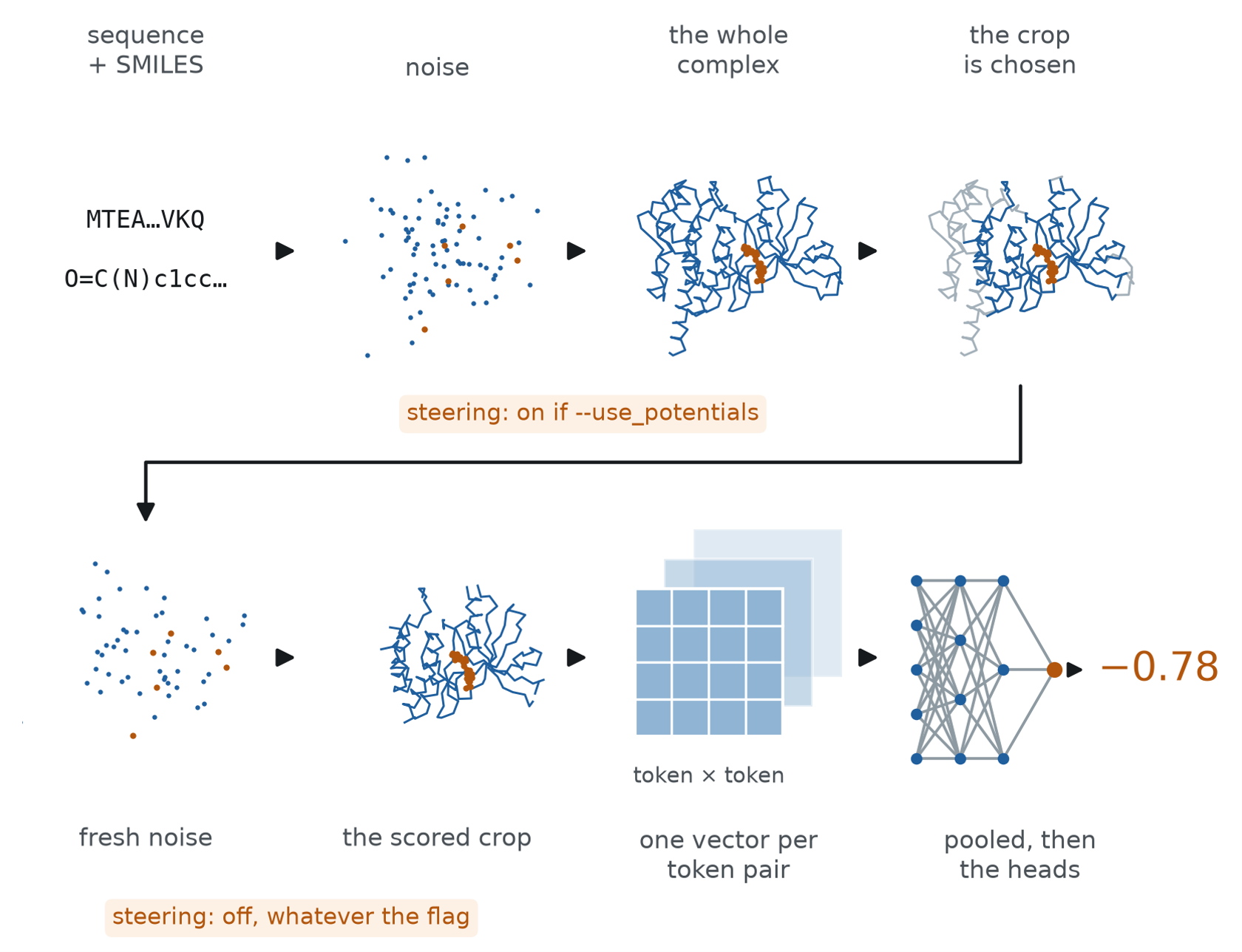
The path one run takes, drawn on an actual 4GIH prediction. The top row is the structure pass and the bottom row the affinity pass. The badges mark where the two folds differ in how they treat the steering potentials. The Cα trace is blue, the ligand’s heavy atoms orange, and the residues that fell outside the crop pale grey.

A complex is predicted from the sequence and the SMILES, starting from noise. AffinityCropper then works outward from the tokens nearest the ligand, adding contiguous runs of residues from each token’s own chain, and stops where the next run would take it past 200 receptor tokens. What it keeps is the crop. The complex is then predicted a second time from fresh noise, using only the residues the cropper kept. This second complex is the one scored for affinity. The crop becomes a token-pair representation, into which the coordinates enter only as binned distances. That representation passes through a stage that mixes information across token pairs. A masked mean reduces it to one vector, which the head reads to produce a single value.
The output file holds the top complex; the affinity value belongs to the bottom one. The two are produced inside one run and are not the same structure. With --use_potentials, the structure pass runs with physical steering, including a chirality correction, while the affinity pass runs with all steering disabled, regardless of the flag setting.

What goes into the affinity head

So what does that second head receive?

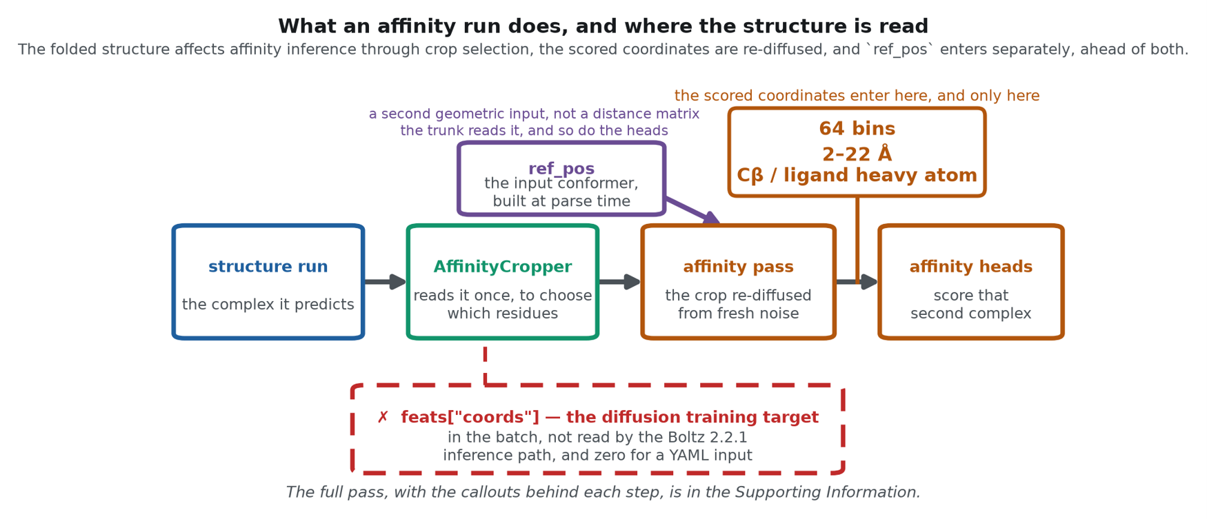
The inference path of a run with affinity. Left to right: the structure pass, the AffinityCropper that reads it once to fix the crop, the affinity pass that re-diffuses the cropped complex from fresh noise with steering disabled, and the head that scores the resulting complex. The orange callout is the only entrance by which the coordinates to be scored reach the head: a matrix of discretized interatomic distances. Each ligand heavy atom forms one token, while each protein residue forms one token represented in this matrix by a single atom. The purple ref_pos is the three-dimensional structure RDKit generates from the SMILES; it arrives through the atom encoder upstream rather than as the distance matrix, and both the trunk and the head read it. The red dashed line is a dead end: the diffusion training target feats["coords"] rides along in the batch, and no inference path of the released checkpoints reads it.

The only route by which the coordinates produced by the structure pass influence the affinity side is through the choice of which residues enter the crop. Past that, the coordinates the head reads are the ones the affinity pass made for itself, and they are read only as binned distances. From here on, we take the scored-coordinate channel and the crop-selection route in turn.

One channel, and what it throws away

The affinity module receives the coordinates to be scored as a distogram. Interatomic distances are clipped to 2–22 Å and discretized into 64 bins, with the 62 bins inside that range each about 0.32 Å wide. The distances are computed using one representative atom per token. Each ligand heavy atom is one token, so the ligand contributes all of its heavy atoms. A protein residue contributes Cβ alone — Cα for glycine.

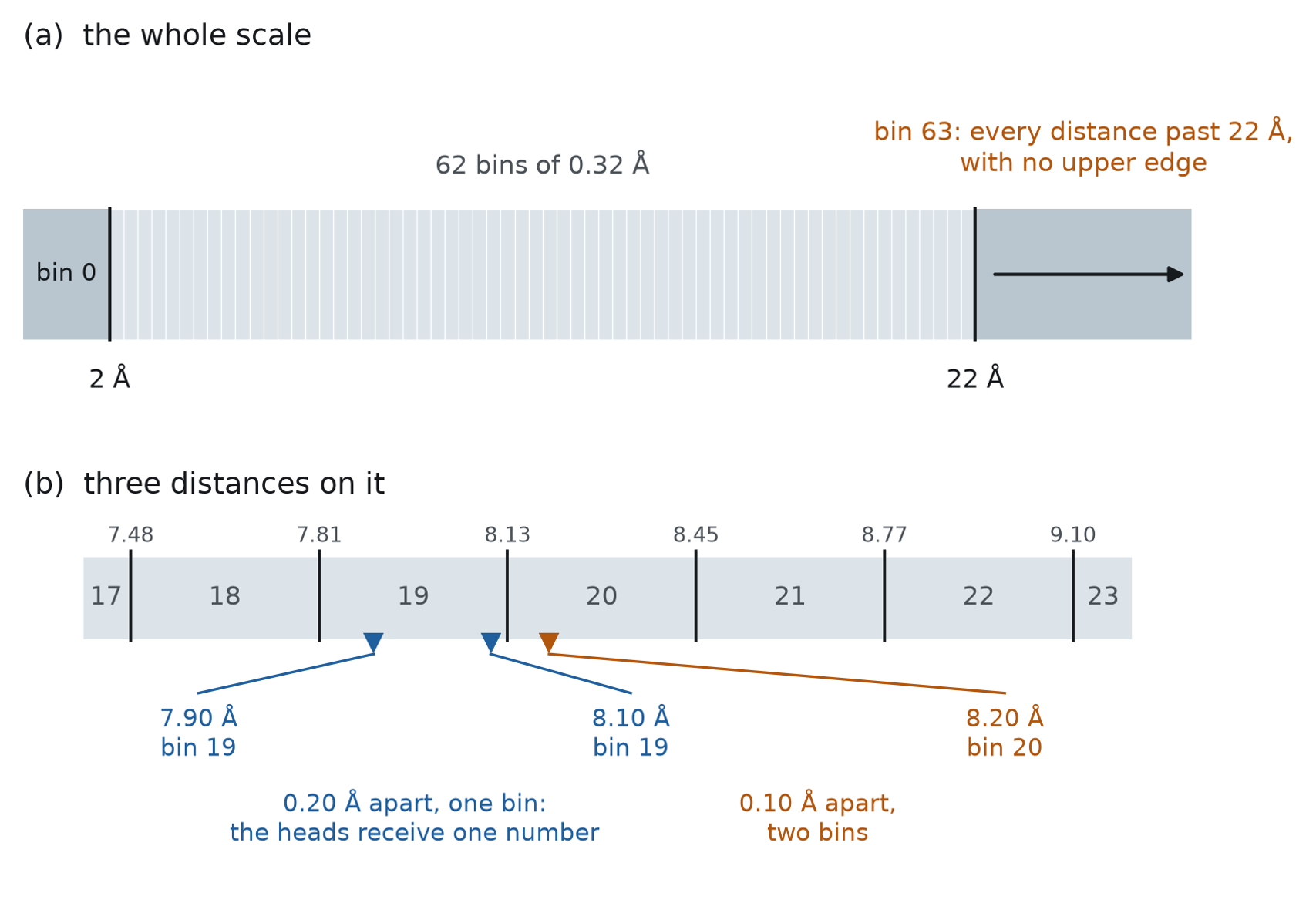
Encoding a distance. (a) The whole scale: the 2–22 Å range contains 62 bins, each 0.32 Å wide; everything closer than 2 Å falls in bin 0, and everything beyond 22 Å in bin 63, which has no upper edge. (b) Ligand↔receptor distances and where they land: 7.90 Å and 8.10 Å are 0.20 Å apart but fall in the same bin, bin 19, and so reach the head as the same encoded value. 8.10 Å and 8.20 Å are only 0.10 Å apart, but they cross a bin boundary and produce different encoded values.

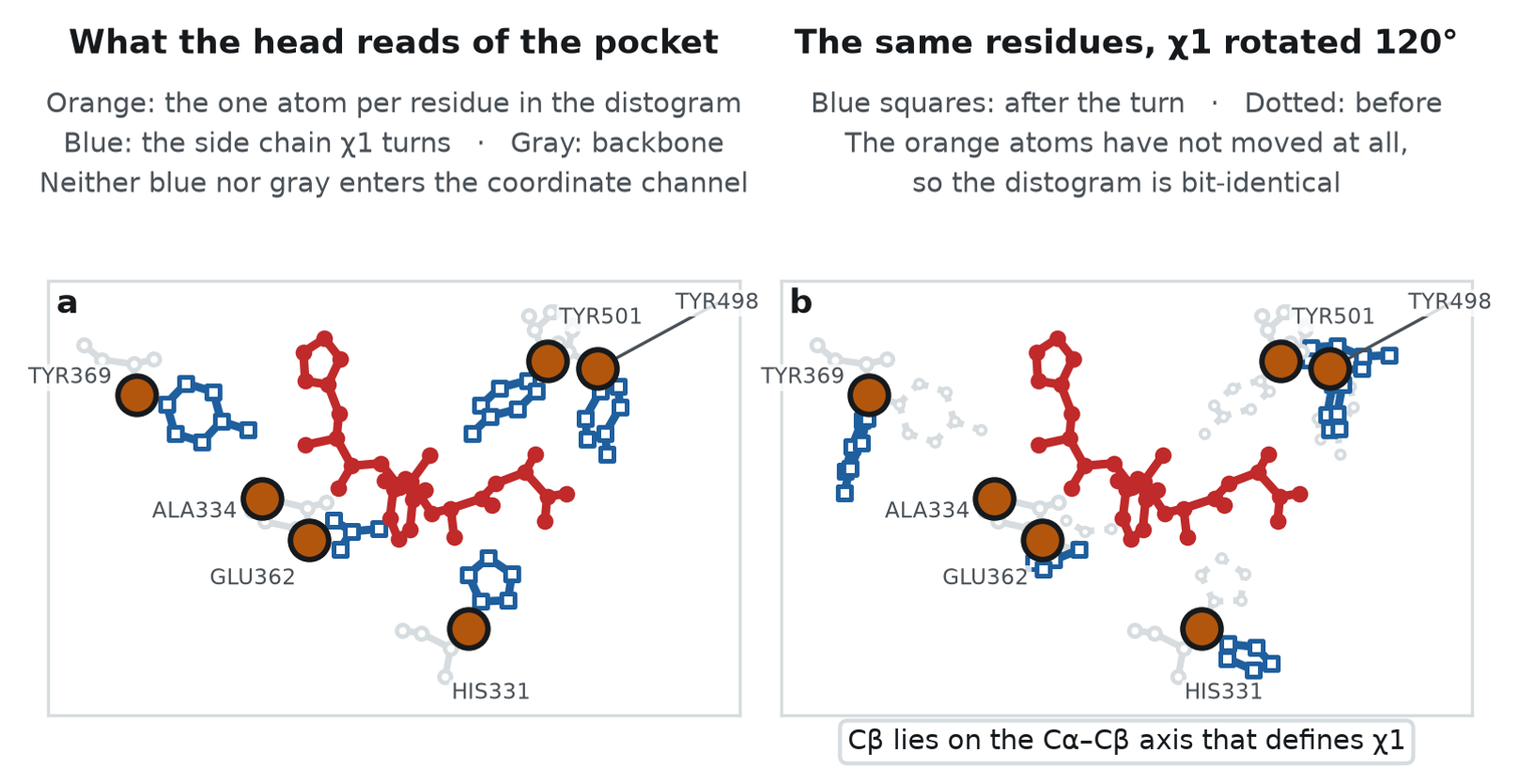
The 4BXK pocket, all-atom. Turn χ1 by 120° and every blue atom moves, while the distogram the heads receive is bit-identical.

Only the orange atoms contribute to the coordinate channel. An atom that is not a token’s representative has no effect on it. Those unread atoms are usually more than 80% of all the atoms in the crop. Because Cβ lies on the χ1 rotation axis, two side-chain rotamers sharing a backbone present this channel with the same input. Receptor-side steric clashes, hydrogen bonds, π-stacking, and similar interactions are not directly represented in this channel. And because it is a distance matrix, the input is invariant under global isometries. So irrespective of the trained weights, rotating, translating, or mirroring the whole complex leaves the input unchanged.
These conclusions come from the source code rather than the measurements. The experiments then confirmed them. We patched Boltz and applied perturbations with analytically zero effects. On every target, the observed changes were zero to within float32 rounding. Jittering the unread atoms by 4 Å or moving them by 10 Å did not change the value.
Atoms are not all this channel drops. The head reads a mean taken over selected token pairs. Ligand↔receptor pairs in both directions and off-diagonal ligand-internal pairs enter that mean; receptor↔receptor pairs and self-pairs do not. Receptor-to-receptor information has not vanished entirely, though — it flows in through a stage inside the stack that rebuilds the pairs.

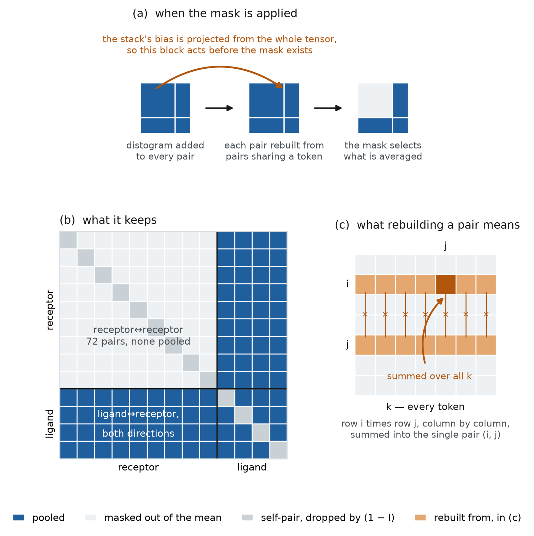
What the pooled mean is taken over, drawn on a schematic of a small receptor and ligand. (a) The order the modules run in. The curved arrow shows how the receptor↔receptor block, left out of the mean, reaches the pairs that survive the mask. (b) The mask cell by cell: ligand↔receptor pairs in both directions and off-diagonal ligand-internal pairs enter the mean, receptor↔receptor pairs and self-pairs do not. (c) One pair-rebuilding step, where pair (i, j) is formed from row i and row j, and row j’s masked entries drop out. The grid is schematic. A real crop typically holds up to 200 receptor tokens against a few dozen ligand tokens, so the excluded block is a far larger share than the figure suggests.

The structure you see is not the structure being scored

The two structures a run produces differ — so how far apart are they? Across the four targets, with six seeds per target, the largest per-target median heavy-atom RMSD was 1.67 Å, and the largest per-target median maximum atomic displacement was 3.35 Å. The ligand is not put somewhere else, though. After receptor superposition, the per-target median ligand-centroid displacement ranged from 0.19 to 1.14 Å. The difference lies in the ligand’s orientation and the arrangement of its atoms, rather than in its overall location. So the reported value is not “the affinity of the pose being displayed.”

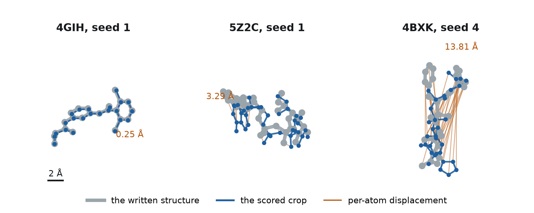
Three folds, the ligand of the written structure beside the ligand the affinity heads scored. The superposition is taken on the receptor — the rigid transform that fits the Cα of the residues the two structures share, applied to the written side; the ligands are not fitted to each other. The orange lines mark atoms displaced by more than that fold’s own receptor residual. The right-hand one is the extreme case: the same place, with the written build turned end for end.

The clearest case in practice is stereochemistry. For some compounds, the structure pass writes out a structure representing a different stereoisomer from that specified by the SMILES. --use_potentials switches on seven physical steering potentials, two of which act on configuration. In our tests, enabling all seven repaired the written structure. But the affinity pass re-diffuses the cropped complex with all steering disabled, so the structure it scores can still represent a different stereoisomer from that specified by the SMILES.

Substituting the pose barely moves the number

With the crop and the upstream representations held bit-identical, we re-scored substituted coordinates through the same heads. The substituted coordinates were taken from four sources: synthetically perturbed poses, poses generated by the same model at other seeds, poses generated by AutoDock Vina, and each entry’s crystallographic pose.
Whichever pose we substituted, the change in predicted affinity stayed under threefold. Changing only the seed and re-running produced a maximum change of 2.4-fold, while the largest single-fold response to any pose substitution was only slightly larger: 2.8-fold versus 2.4-fold, both on 4BXK. When averaged over the six folds, the re-folding and pose-substitution responses were of the same order.

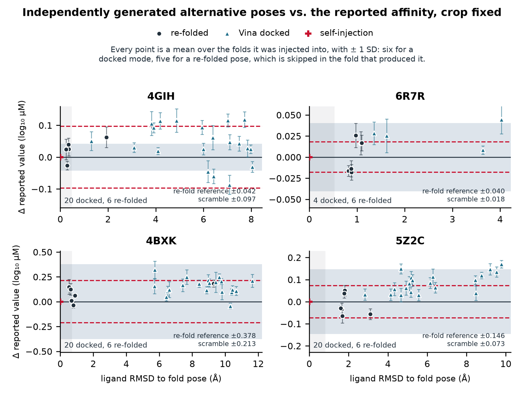
Independently generated poses injected through a fixed crop. The horizontal axis is the distance from the pose scored by that fold. The band is that target’s re-fold reference — the spread from re-running the identical input — and the red cross at the origin is the self-injection control. Each panel is scaled to its own target, so the heights are not comparable across them.

What does move it

intervention	range of \|Δ\|（log₁₀(μM))	maximum fold change
pose substituted at a fixed crop	0.015–0.445	2.8×
which residues are cropped	0.56–1.99	98×
which ligand is bound	0.48–2.00	100×
one pocket residue → alanine	0.14–2.40	251×

The four rows do not count the same thing. The pose row summarizes 64 docked modes evaluated across six folds each; the crop and ligand rows each summarize one fold per configuration; and the alanine row summarizes 12 substitutions evaluated across six folds each.

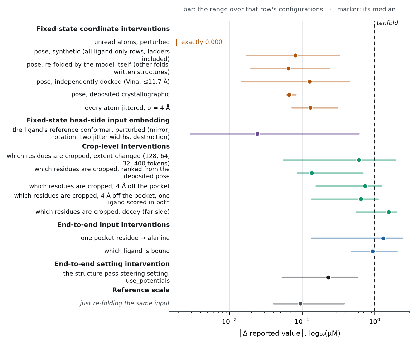
Every intervention in the study on a common axis, grouped by where it enters the pipeline. The dashed line is tenfold, and the bottom row is re-folding the identical input.

The decoy crop keeps the requested receptor-token count at 200 and changes only the crop’s location, thereby changing its composition rather than its size.
The same pattern held across twenty complexes selected without reference to the four studied in detail, with three seeds per complex: ligand-only perturbations stayed under 0.19 log units, or less than 1.6-fold, in every complex, while changing what was cropped moved the predicted affinity by more than a hundredfold in some complexes.

What is the structure-pass pose good for?

The structure-pass pose is not irrelevant — it is routed differently. The cropper ranks residues by their distance to the ligand, so the coordinates produced by the structure pass determine which residues are passed to the affinity pass. The affinity pass then rebuilds its features, trunk representation, and ligand geometry from that selection.
On every target, displacing the ligand by 4 Å before crop selection produced a larger response than substituting any pose after the crop had been fixed.

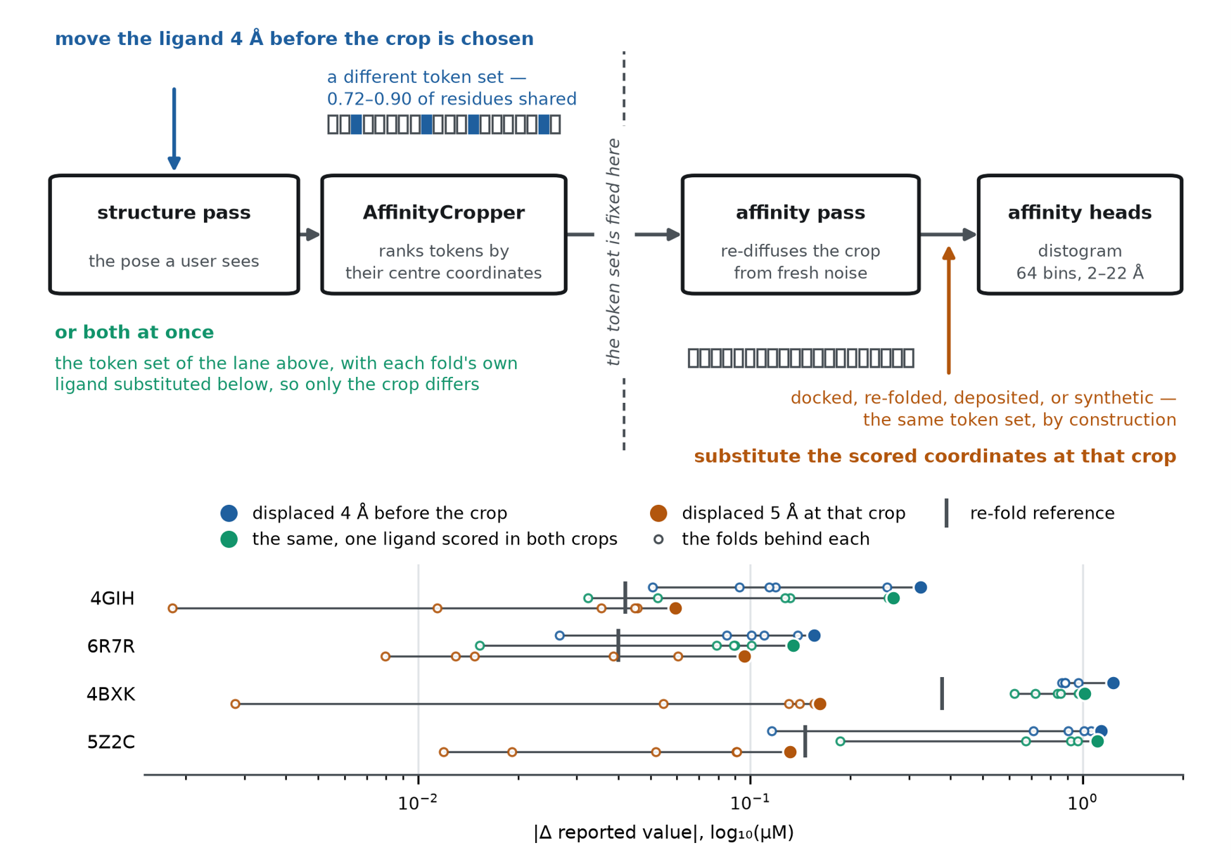
The same operation on either side of the cropper. Above, where each enters; below, the size of the response, with each target’s re-fold reference as a vertical tick. Open circles are the six folds of each series, and the filled marker the largest of them. The two ladders were run at different rungs, 4 Å before the crop and 5 Å after it.

Notes for anyone using the affinity prediction

Do not read the affinity value as a score for the pose drawn beside it. Do not expect a better pose to buy a better prediction while the crop is held fixed. In virtual screening, the point to watch is that AffinityCropper selects the crop from each ligand’s own fold. That is, two compounds in one library are not guaranteed to be scored against the same set of residues.
To put a number on that, we took 32 TYK2 inhibitors whose binding activities are reported in ChEMBL and ran each against 4GIH under two crops: the crop Boltz produces in an ordinary run, and a decoy crop moved to the side of the receptor farthest from the ligand. Under the decoy crop, the predicted affinities shifted by an average of +1.10 log units, and 90% shifted toward weaker predicted binding. Taking the 20 compounds with pChEMBL values of 7.0 or above as active, the ordinary crop predicted 17 of them to bind more tightly than 1 μM, whereas the decoy crop predicted only 10 to do so. A decoy crop is not something an ordinary run produces, but it shows how strongly crop composition affects the predicted affinity.
One last thing: this work measured sensitivity to the pose, and that is not a claim that the affinity value is of no use. It measured how far the value moves, one complex at a time; it did not test the ability to rank a library. Even among the 32 compounds above, the ranking by predicted value matched the experimental activity labels better than expected by chance (label-shuffle p ≈ 0.002). At screening scale, pose quality has been reported to matter for ranking [2]. A response of one tenth of a log unit within a single complex and the ordering of tens of thousands of compounds belong to different scales of evaluation. A small response on the first scale does not imply poor performance on the second.

Scope

The claims here are limited to what the complexes and conditions we examined support. We evaluated four complexes in detail, at six seeds each. The coordinate battery and decoy-crop experiments added twenty complexes to the four examined in detail, bringing the total to twenty-four. The coordinate battery alone also covered three systems outside that set. Three of the four targets examined in detail were also chosen from complexes for which Boltz got the ligand stereochemistry wrong at every seed we examined. This work is based on the open-source Boltz 2.2.1; other versions and forks were not examined.

References

Bret, G.; Sindt, F.; Rognan, D. Assessing Boltz-2 performance for the binding classification of docking hits. J. Chem. Inf. Model. 2026, 66, 1511–1521. DOI: 10.1021/acs.jcim.5c02630.
Furui, K.; Ohue, M. Boltzina: efficient and accurate virtual screening via docking-guided binding prediction with Boltz-2. arXiv 2025, arXiv:2508.17555v1. DOI: 10.48550/arXiv.2508.17555.
Kim, J.; Correy, G. J.; Hall, B. W.; Rachman, M. M.; Mailhot, O.; Togo, T.; Gonciarz, R. L.; Jaishankar, P.; Neitz, R. J.; Hantz, E. R.; Doruk, Y. U.; Stevens, M. G. V.; Diolaiti, M. E.; Reid, R.; Gopalkrishnan, S.; Krogan, N. J.; Renslo, A. R.; Ashworth, A.; Shoichet, B. K.; Fraser, J. S. Large scale prospective evaluation of co-folding across 557 Mac1–ligand complexes and three virtual screens. bioRxiv 2025. DOI: 10.64898/2025.12.25.696505.

Preprint: Pose-to-Affinity Information Flow in Boltz-2: Pathways and Response Magnitude. DOI: 10.26434/chemrxiv.15006767
Source code and all result files: https://github.com/xeureka-research/boltz2-affinity-pose-sensitivity